A number is not a plant trait
A repeat camera produces images. An image-processing workflow produces numbers. But the step between those two statements is easy to overlook, particularly when a smooth seasonal curve appears to describe greenness, flowering, senescence, or stress with remarkable clarity. Repeat photography is valuable because it turns a fixed viewpoint into a record of change. A camera can observe the same crop, grassland, forest canopy, shoreline, or snow-covered slope many times each day. The resulting images retain the context of each observation, while image-derived indices provide concise time series that are easier to compare, plot, and connect with other observations. But an index is not a direct measurement of plant condition. It is a numerical summary of selected pixel values, calculated using a particular formula, region of interest, and image-processing workflow. Its scientific usefulness depends on whether changes in that summary can be meaningfully related to the process we are interested in.
What does an index actually measure?
When observing vegetation, we often use the Normalized Difference Vegetation Index, or NDVI. NDVI combines information from the red and near-infrared portions of the electromagnetic spectrum. It is based on a relatively simple principle: green leaves absorb much of the incoming red light while reflecting a relatively large proportion of near-infrared light.
As a result, dense, healthy, green vegetation often has relatively low reflectance in the red band and relatively high reflectance in the near-infrared band. When the difference between the two is large relative to their sum, NDVI is high. Values approaching 0.8 are commonly associated with dense green canopies, although the exact value depends on the sensor, target, viewing conditions, and processing method. Lower values can indicate sparse vegetation, senescence, bare soil, water, snow, or other surfaces.
The important point is that NDVI does not measure plant health directly. It is calculated from the relationship between two measured signals. The interpretation comes afterwards.
The same principle applies to RGB indices, even though the information they use is different.
From pixels to colour channels
A typical RGB image is made up of pixels. Each pixel contains a red, green, and blue value. In a standard 8-bit JPEG image, these values commonly range from 0 to 255. In most cameras, the values are digital numbers produced after the sensor, lens, exposure settings, white balance, compression, and internal image processing have shaped the incoming light.
A pixel representing a strongly green part of a plant may, for example, have a relatively high green value and lower red and blue values.
However, these numbers are influenced not only by the target itself, but also by the conditions under which it was observed. A vegetation canopy may look different because leaves have emerged, but it may also look different because the sun is lower, a cloud has passed, the camera has adjusted its exposure, a shadow has moved, or the region of interest contains more sky or soil than it did previously.
This does not make repeat photography unsuitable for science. It makes careful acquisition and interpretation necessary.
The strength of repeat photography often lies in its ability to describe relative change at one site, from a stable viewpoint, over time. But there is an important caveat.
I once designed a field camera that automatically adjusted white balance and other image parameters, optimising each photograph as it was taken. The result was impressive. The camera produced consistently crisp and visually pleasing images, even under less-than-ideal conditions. However, when I calculated indices from those images, something unexpected happened. The index values were remarkably similar from one image to the next. The camera was doing such a good job of adjusting each image to produce a visually consistent result that it was also reducing some of the variation that the monitoring system was intended to capture.
This is a useful reminder that a better-looking image is not necessarily a better measurement.
Regions of interest (ROI)
Images are usually recorded as rectangles. Most of the things we want to observe, however, are not rectangular and may occupy only part of the camera’s field of view, or FOV.
For this reason, indices are usually calculated within a region of interest, commonly abbreviated as ROI. The ROI is the selected part of an image intended to represent the target. It might cover a crop canopy, a section of grassland, a tree crown, a forest stand, or another clearly defined part of the scene.
ROI selection is therefore a scientific decision, not a cosmetic one.
Including sky, soil, buildings, water, shadows, or moving objects can alter the resulting time series. A useful ROI represents the target as consistently as possible, remains stable through time, and is documented so that another user can understand what was included. For example, if we want to monitor a maize field, we would generally try to exclude shadows cast by nearby trees. Otherwise, changes in the position or length of those shadows could be interpreted as changes in the maize canopy. In the picture below you can see the ROIs of a PhenoCam monitoring an almond orchard in Spain as an example.
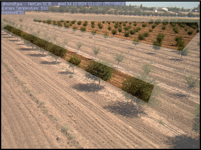
Figure 1: Example images of ROI application in a PhenoCam in Spain monitoring an almond orchard. The ROI is applied over the most dense canopy areas.
When targets are heterogeneous, it can be useful to define more than one ROI. Separate regions might represent different crop treatments, canopy layers, species, slope positions, or parts of a field. The resulting curves should not automatically be treated as interchangeable. Their comparability depends on how the targets are defined and whether they were observed under comparable conditions.
Common RGB indices
As discussed above, NDVI requires information from the near-infrared part of the spectrum. Standard repeat-photography cameras, however, usually use an RGB sensor designed to record visible light, often with filtering that limits the near-infrared response.
One of the most widely used indices for phenological repeat photography is the Green Chromatic Coordinate, usually called GCC. It is commonly calculated as:
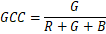
By expressing the green channel relative to the combined red, green, and blue signal, GCC can reduce sensitivity to overall brightness changes and make seasonal changes in canopy greenness easier to track.
Other indices use different combinations of the same three colour channels. The Red Chromatic Coordinate, or RCC, expresses the relative contribution of red. Excess Green, or ExG, emphasises green relative to red and blue. The Green-Red Vegetation Index, or GRVI, compares green and red values.
Each formula highlights different aspects of visible colour, and each can respond differently to illumination, camera type, target structure, and background.
There is no universally best index when monitoring vegetation. The appropriate choice depends on the target, the scientific question, the camera, and the processing workflow. In many cases, it is more useful to understand what an index actually summarises than to search for a universally optimal formula.
Timing matters
The timing of image acquisition can strongly affect RGB time series. Morning and evening images often contain long shadows and stronger colour casts because the composition of incoming light changes with solar angle and atmospheric conditions. Midday images may reduce some shadow effects, but they can introduce other problems, including glare, saturation, and strong directional illumination.
Overcast conditions can provide more diffuse light, but they are not necessarily equivalent to sunny conditions. The important point is that the same scene can produce different pixel values simply because it was photographed under different illumination.
For this reason, many workflows select images from a consistent time window, calculate daily summaries, filter unsuitable images, or apply smoothing methods to reduce short-term noise. These choices should be documented because they influence both the shape and timing of the final curve.
Repetition does not remove uncertainty. It makes uncertainty visible and, with a good workflow, manageable.
A long image record allows us to identify outliers, abrupt camera changes, lens obstructions, snow cover, management events, and periods when the target was not observed under comparable conditions. That information is part of the dataset, not merely a nuisance to be removed.
From index to phenology
For vegetation applications, a seasonal GCC curve may rise during green-up, reach a peak during mature canopy conditions, and decline during senescence.
Researchers can use features of that curve to estimate transition dates, compare seasonal timing among sites, or relate visible canopy development to temperature, flux measurements, field observations, drone imagery, and satellite products.
But the curve does not directly reveal the date on which every leaf emerged, nor does it directly measure the amount of chlorophyll in a canopy. It describes a repeatable pattern in the camera record.
Connecting that pattern to a biological event requires field knowledge, reference observations, and an explicit interpretation framework.
This distinction is particularly important in crops and managed landscapes. Flowering, mowing, grazing, irrigation, tillage, harvest, residue cover, and changes in soil background can all alter an RGB index. These effects may be scientifically useful, but they should not automatically be interpreted as a generic measure of vegetation health.
Visible colour can sometimes provide useful information about vegetation condition. A green canopy may be actively growing or photosynthetically active, while yellowing or browning may indicate senescence, drought, nutrient limitation, disease, disturbance, or normal seasonal change. These interpretations depend on the species, phenological stage, management context, and other available evidence.
This is where repeat photography can be particularly powerful.
For example, indices can work very well when the goal is to compare two fields in a management experiment. They can also be useful for examining patterns of drying of canopies across a larger region, such as a province. In these cases, the index does not need to be a universal measure of plant condition. It needs to provide a consistent and interpretable signal that allows observations to be compared within a well-defined study.
A useful summary, not a substitute
RGB indices are valuable because they turn a large archive of images into interpretable time series. They support visual inspection, reveal seasonal patterns, and make it possible to compare repeated observations in a structured way.
But the index is not the observation itself.
It is a summary of the observation.
The image, the ROI, the acquisition conditions, and the processing workflow all remain part of the evidence. If that context is removed, a number can easily appear to mean more than it actually does.
This is why repeat RGB photography works best as a documented observation system. Stable geometry, suitable camera settings, consistent timing, image-quality control, transparent processing, and meaningful links to field measurements all matter.
A number can be useful. A smooth curve can be informative. But neither becomes a plant trait simply because it looks convincing.
Explore further:
- Richardson, A. D., Jenkins, J. P., Braswell, B. H., Hollinger, D. Y., Ollinger, S. V., and Smith, M. L. (2007). Use of digital webcam images to track spring green-up in a deciduous broadleaf forest. Oecologia, 152, 323–334. https://doi.org/10.1007/s00442-006-0657-z
- Sonnentag, O., Hufkens, K., Teshera-Sterne, C., Young, A. M., Friedl, M., Braswell, B. H., Milliman, T., O’Keefe, J., and Richardson, A. D. (2012). Digital repeat photography for phenological research in forest ecosystems. Agricultural and Forest Meteorology, 152, 159–177. https://doi.org/10.1016/j.agrformet.2011.09.009
- Woebbecke, D. M., Meyer, G. E., Von Bargen, K., and Mortensen, D. A. (1995). Color indices for weed identification under various soil, residue, and lighting conditions. Transactions of the ASAE, 38(1), 259–269. https://doi.org/10.13031/2013.27838
- Hufkens, K., Friedl, M. A., Sonnentag, O., Braswell, B. H., Milliman, T., and Richardson, A. D. (2012). Linking near-surface and satellite remote sensing measurements of deciduous broadleaf forest phenology. Remote Sensing of Environment, 117, 307–321. https://doi.org/10.1016/j.rse.2011.10.006
Leave a Reply