The most disappointing moment in field data acquisition is when you realize that the data you collected are full of errors or even useless for your objectives. Having been a drone pilot for the better part of two decades, I can tell you that a small power spike erasing an SD card full of camera data or dust covering a camera lens are not things that have happened only once. In this article, I would like to look beyond these mishaps and take a more systematic look at data quality in proximal sensing.
Most bad data begin in the field
A well-designed algorithm cannot recover information that was never recorded properly, reconstruct a shifted camera view without evidence of the original geometry, or determine whether a suspicious soil-sensor value reflects a real change or poor sensor contact. Data quality is not something that begins after fieldwork. It starts when the system is designed, installed, and maintained.
This is especially clear in proximal sensing, where we often collect our own data rather than simply accessing datasets collected by others. Sensors operate close to their targets and to the messy realities of the field: mud, dust, rainfall, vegetation growth, insects, spider webs, birds, rodents, loose cables, power loss, unstable mounts, intermittent communication, changing illumination, and human activity. These are not marginal inconveniences. They are part of the measurement environment.
The field has a sense of humor
Let’s be honest, most of these mishaps have their own irony. We might spend weeks designing the perfect distribution of cameras across a region, only to find that a spider web covers one lens from the very day a rapid phenological change occurs. Our key statistics then fail to capture the event as expected. A raindrop may produce a bright patch that looks like a target feature. A growing branch may slowly enter a camera’s field of view. A cow may rub against a mounting pole or nibble on cables. A battery may fail after several cloudy days and insufficient solar charging. A sensor may continue sending the same value after losing contact with the soil. And have we even started talking about duckweed blooms in rice fields?
These examples are familiar because field systems are long-lived and exposed to whatever nature throws at them. Treating them as expected failure modes leads to better designs. Weatherproof housing, robust mounting, cable protection, power margins, local storage, health checks, reference images, maintenance records, and automated alerts can prevent or at least document many problems.
Quality begins with design
Choose a system that is appropriate for the expected conditions. I have seen studies where a microphone sensor was deployed in the field in a simple zipper bag. That can work, of course, but the most advanced sensor is not always the best choice if it cannot be powered, maintained, protected, or calibrated at the intended site. Plan for heat, cold, humidity, dust, rain, wind, insects, animals, vandalism, vegetation growth, site access, and communication failures.
Before deployment, define what acceptable data look like. Set expected ranges, sampling intervals, minimum image quality, required metadata, storage procedures, and criteria for flagging observations. This makes later quality control more consistent and easier to automate.
I know this may all sound rather abstract, especially when you are just starting to deploy a new system. My suggestion is simple: run a test. Buy a few sensors or take your spectrometer into the parking lot and make some measurements outside your actual study. Look at the data. What looks good? What could break your analysis? Tests are great, so always run one before collecting data for a real study.
Inspect the first data
The first hours and days after installation are particularly valuable. Review the actual outputs rather than assuming that a successful installation has produced useful measurements. Check camera framing, sensor orientation, timestamps, time zones, sampling intervals, file names, connectivity, battery behavior, and the relationship between recorded values and known conditions. Is the calibration panel in the field of view? Does your probe move in the wind? Is water collecting around a cable connector?
For long time series, keep up this habit. Plot recent data alongside earlier observations. Do they match your expectations? Inspect random images, not just selected good examples. Compare sensor streams after maintenance. Use simple dashboards where possible. The aim is to detect changes in the measurement system before they are mistaken for changes in the target.
Flags preserve evidence
A quality flag does not have to mean deletion. It can indicate that an observation was affected by rain, snow, fog, lens obstruction, sensor maintenance, a communication gap, a moved camera, a questionable calibration period, or an unknown condition. Flagging retains the original observation and documents why a user should treat it cautiously. Much of this can be automated. However, never delete outliers from your original dataset. Flag them as suspicious and exclude them from your analysis if you can justify doing so. Deleting outlier rows from an Excel sheet is bad practice because the original dataset and your decisions may no longer be reproducible. This approach is preferable to quietly replacing, smoothing, or deleting inconvenient records. It preserves provenance and allows later users to apply different filters depending on their research question.
Imagine monitoring a rice field. As an agronomist, you might want to exclude images with thick fog, rain, or strong wind from your vegetation-phenology analysis. However, these images could be extremely valuable to a colleague studying exactly those weather conditions. A maintenance period may be unsuitable for analyzing long-term trends but useful for diagnosing a sensor problem.
Common checks, different sensors
Camera systems need checks for blur, obstruction, reflections in the field of view, exposure changes, night images, shadows, scene movement, region-of-interest stability, and missing files. Thermal systems also need attention to calibration status, reference targets, reflected radiation, and thermal drift. Weather stations should be checked for insects under radiation shields, dust build-up, and vandalism. Soil sensors need checks for installation depth, soil contact, response range, and changes after wetting or drying. Spectral systems need reference standards, consistent measurement geometry, and checks for saturation and illumination conditions.
The exact rules should be sensor-specific, but the principle is general: quality control must reflect the measurement physics and the field environment.
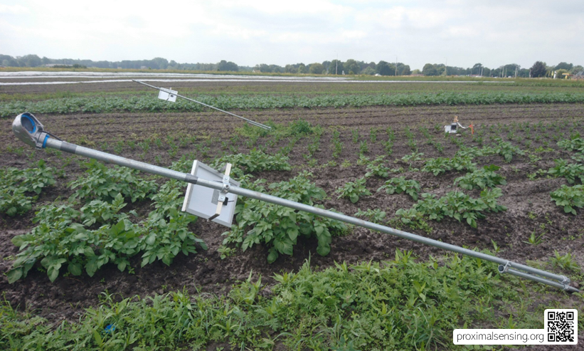
Figure 1. Broken cameras in one of our field setups, resulting in a data gap of several weeks. SD cards and batteries seem to have been tempting targets for thieves. These things happen in fieldwork, and the important thing is to account for them in a good data quality management plan.
Quality is a shared workflow
Data quality improves when it is considered throughout the life of a project. Field teams can record maintenance and local conditions. Hardware designers can build in health indicators. Data managers can preserve raw files and metadata. Analysts can identify anomalies in time series. Domain experts can distinguish an unlikely value from an unusual but genuine environmental event.
A good workflow makes these roles visible. It creates a clear path from observation to flagged data to reviewed product, with decisions documented along the way.
The result is trustworthy data
Data quality is not an administrative burden added after the scientific work. It is one of the ways scientific work becomes trustworthy. A dataset with known limitations, visible flags, retained raw observations, and documented interventions is more useful than a neat dataset whose history has been erased and that simply looks perfect. Proximal sensing often produces dense, long-lived records. The more automated a system becomes, the more important it is to maintain a clear connection between the data stream and the field conditions that produced it.
Explore further:
- Schmidt, L., Schäfer, D., Geller, J., Lünenschloß, P., Palm, B., Rinke, K., Rebmann, C., Rode, M., and Bumberger, J. (2023). System for automated quality control (SaQC) to enable traceable and reproducible data streams in environmental science. Environmental Modelling & Software, 169, 105809. https://doi.org/10.1016/j.envsoft.2023.105809
- Bumberger, J., Abbrent, M., Brinckmann, N., Hemmen, J., Kunkel, R., Lorenz, C., Lünenschloß, P., Palm, B., Schnicke, T., Schulz, C., van der Schaaf, H., and Schäfer, D. (2025). Digital ecosystem for FAIR time series data management in environmental system science. SoftwareX, 29, 102038. https://doi.org/10.1016/j.softx.2025.102038
Leave a Reply